Visualize your data: DOs and DONT's
Some design principles
The Minard Map


Matplotlib & Seaborn
Matplotlib
						import matplotlib.pyplot as plt
						fig = plt.figure()

Matplotlib
						import matplotlib.pyplot as plt
						fig, ax = plt.subplots()

Matplotlib
						import matplotlib.pyplot as plt
						fig, axes = plt.subplots(1, 2, figsize=(12, 4))

Matplotlib
									import matplotlib.pyplot as plt
									fig, axes = plt.subplots(1, 2, figsize=(4, 8))
									x = [0.2, 0.6]
									y = [0.4, 0.5]
									axes[0].scatter(x, y, s=60)
									axes[1].bar(x, y, width=0.1)

Matplotlib
									import matplotlib.pyplot as plt
									fig, axes = plt.subplots(1, 2, figsize=(4, 8))
									x = [0.2, 0.6]
									y = [0.4, 0.5]
									axes[0].scatter(x, y, s=200, color="r")
									axes[1].bar(x, y, width=0.1)
									axes[1].set_xticks([])
									axes[1].set_title("a barchart", fontsize=16)
Modify overall aesthetics in plot call.
Modify individual elements via set_element(attribute).

Seaborn
A high-level interface to Matplotlib for statistical analyses. Get inspiredy by the gallery.
									import seaborn as sns
									sns.set_theme(style = "whitegrid")
									iris = sns.load_dataset("iris")
									iris = pd.melt(iris, "species", var_name = "measurement")
									fig, ax = plt.subplots()
									sns.stripplot(
										data = iris,
										x = "value",
										y = "measurement",
										hue = "species",
										dodge = True,
										alpha = .25,
										ax = ax
									)
									ax.set_ylabel("")

Why Matplotlib?
... Matplotlib is a pain in the ass to learn.
I know Matplotlib.
Great synergy with seaborn.
Other packages like networkx build on it.
Matplotlib offers very fine control over all figure elements.
For publication-level plots it pays off to learn Matplotlib.
Overview: Python plotting packages
| package | style | pro | con |
|---|---|---|---|
| matplotlib | object oriented | very customizable, many extensions | very complex |
| seaborn | declarative | very sensible defaults, easy(er) to use | less customizable, but can fall back to matplotlib |
| plotly | declarative | easy to use, made for interactive visualizations, also available for R | less customizable, getting used to web apps might take some getting used to |
| altair | declarative | easy to use | less customizable |
| bokeh | grammar of graphics | rather straight forward to use, can handle very big data | less customizable, getting used to web apps might take some getting used to |
| plotnine | grammar of graphics | similar to ggplot2 in R, straight forward to use | less customizable |
Plot types
| dim 1 | dim 2 | type | function |
|---|---|---|---|
| numerical | - | histogram | sns.histplot() |
| numerical | categorical | bar chart | sns.barplot() |
| numerical | time | time series | ax.plot() |
| numerical | numerical | scatter plot | sns.scatterplot() |
Example study
"New conceptions of truth foster misinformation in online public political discourse"
(-) Conceptions of "truth" splinter into two distinct camps.
(-) "Truth-seeking" aims to uncover factual information and update one's beliefs.
(-) "Belief-speaking" conceptualizes truth as "authenticity" and "speaking one's mind".
(-) We measure "truth-seeking" and "belief-speaking" in tweets by U.S. Congress Members.
Example data
"New conceptions of truth foster misinformation in online public political discourse"


Histogram: number of tweets per account
									import matplotlib.pyplot as plt
									import seaborn as sns
									users = pd.read_csv("users.csv")

									sns.histplot(
										data=users,
										x="tweet_count"
									)

Adapt aspect ration to data
									fig, ax = plt.subplots(figsize=(8, 4))

									sns.histplot(
										data=users,
										x="tweet_count",
										ax=ax
									)

Choose intuitive bin width
									fig, ax = plt.subplots(figsize=(8, 4))

									sns.histplot(
										data=users,
										x="tweet_count",
										ax=ax,
										bins=range(0, 3510, 250),
										shrink=0.8
									)

De-cluttering
									fig, ax = plt.subplots(figsize=(8, 4))

									sns.histplot(
										data=users,
										x="tweet_count",
										ax=ax,
										bins=range(0, 3510, 250),
										shrink=0.8,
										edgecolor=None
									)
									ax.spines["top"].set_visible(False)
									ax.spines["right"].set_visible(False)
									ax.set_xlabel("Tweet count", fontsize=16)
									ax.set_ylabel("User count", fontsize=16)

Barchart: two categories
									fig, ax = plt.subplots(figsize=(8, 4))

									sns.barblot(
										data=belief_speaking,
										x="proportion",
										y="time_period",
										hue="party",
										ax=ax
									)

Use known metaphors
									fig, ax = plt.subplots(figsize=(8, 4))

									sns.barblot(
										data=belief_speaking,
										x="proportion",
										y="time_period",
										hue="party",
										ax=ax,
										palette=["#0015BC", "#FF0000"],
										hue_order=["Democrat", "Republican"]
									)

De-cluttering
									sns.barblot(
										data=belief_speaking,
										x="proportion",
										y="time_period",
										hue="party",
										ax=ax,
										palette=["#0015BC", "#FF0000"],
										hue_order=["Democrat", "Republican"]
									)
									ax.spines['right'].set_visible(False)
									ax.spines['top'].set_visible(False)
									ax.legend(frameon=False, fontsize=16)
									ax.set_ylabel("")
									ax.set_xlabel("% of Tweets", fontsize=16)
									ax.tick_params(axis='both', labelsize=12)

Alternative category representation
									sns.barblot(
										data=belief_speaking,
										x="proportion",
										y="party",
										hue="time_period",
										ax=ax,
										palette=[(0.5, 0.5, 0.5), (0.2, 0.2, 0.2)],
										hue_order=["2010 to 2013", "2019 to 2022"]
									)

Time-series: number of tweets
									counts = pd.read_csv(
										"tweet_counts.csv",
										parse_dates = ["date"]
									)
									counts = counts.set_index("date")
									dem = counts[counts["party"] == "Democrat"]
									rep = counts[counts["party"] == "Republican"]

									fig, ax = plt.subplots(figsize = (9, 4))
									ax.plot(
										dem.index,
										dem["tweet_count"],
										color = "#0015BC",
									)

Rolling average
									counts = counts.set_index("date")
									dem = counts[counts["party"] == "Democrat"]\
										.rolling("90D").mean()
									rep = counts[counts["party"] == "Republican"]\
										.rolling("90D").mean()

									fig, ax = plt.subplots(figsize = (9, 4))
									ax.plot(
										dem.index,
										dem["tweet_count"],
										color = "#0015BC",
									)

Labels & de-cluttering
									fig, ax = plt.subplots(figsize = (9, 4))
									ax.plot(
										dem.index,
										dem["tweet_count"],
										color = "#0015BC",
										label="Democrat"
									)
									ax.set_ylabel("Tweet count", fontsize=12)
									ax.legend(frameon=False, loc=6)
									ax.spines['right'].set_visible(False)
									ax.spines['top'].set_visible(False)

Annotations
									p_elections = [pd.to_datetime(date) for\
									            date in ["2012-11-06", "2016-11-08", "2020-11-03"]]
									s_elections = [pd.to_datetime(date) for\
									            date in ["2013-11-05", "2014-11-04", "2015-11-03",
									                     "2017-11-07", "2018-11-06", "2019-11-05"]]
									for el in p_elections:
									    ax.plot([el, el], [0, 750], color="k")
									for el in s_elections:
									    ax.plot([el, el], [0, 600], "--", color="grey")

									ax.text(pd.to_datetime("2013-07-01"), 650,
									        "Congress elections", color="grey", fontsize=12)
									ax.text(pd.to_datetime("2015-03-01"), 800,
									        "Presidential elections", color="k", fontsize=12)

Scatterplot: followers vs. following
									fig, ax = plt.subplots(figsize = (7, 4))
									sns.scatterplot(
										data = users,
										x = "followers_count",
										y = "following_count",
										hue = "party",
										palette = ["#0015BC", "#FF0000"],
										hue_order = ["Democrat", "Republican"],
										ax = ax
									)

Logarithmic axis scales
									fig, ax = plt.subplots(figsize = (7, 4))
									sns.scatterplot(
										data = users,
										x = "followers_count",
										y = "following_count",
										hue = "party",
										palette = ["#0015BC", "#FF0000"],
										hue_order = ["Democrat", "Republican"],
										ax = ax
									)
									ax.set_yscale("log")
									ax.set_xscale("log")

Labels & de-cluttering
									sns.scatterplot(
										data = users,
										x = "followers_count",
										y = "following_count",
										hue = "party",
										palette = ["#0015BC", "#FF0000"],
										hue_order = ["Democrat", "Republican"],
										ax=ax
									)
									ax.set_xlabel("followers", fontsize=12)
									ax.set_ylabel("following", fontsize=12)
									ax.legend(frameon=False, fontsize=12)
									ax.spines['right'].set_visible(False)
									ax.spines['top'].set_visible(False)

Adding another data dimension
									sns.scatterplot(
										data = users,
										x = "followers_count",
										y = "following_count",
										size = "N_tweets",
										hue = "party",
										palette = ["#0015BC", "#FF0000"],
										hue_order = ["Democrat", "Republican"],
										alpha = 0.3,
										linewidth = 0,
										ax = ax
									)
									ax.legend(frameon = False, loc = 9, fontsize = 12,
										bbox_to_anchor = [1.2, 0.9, 0, 0],
									)

Visualizing words: wordcloud

Visualizing words: scattertext

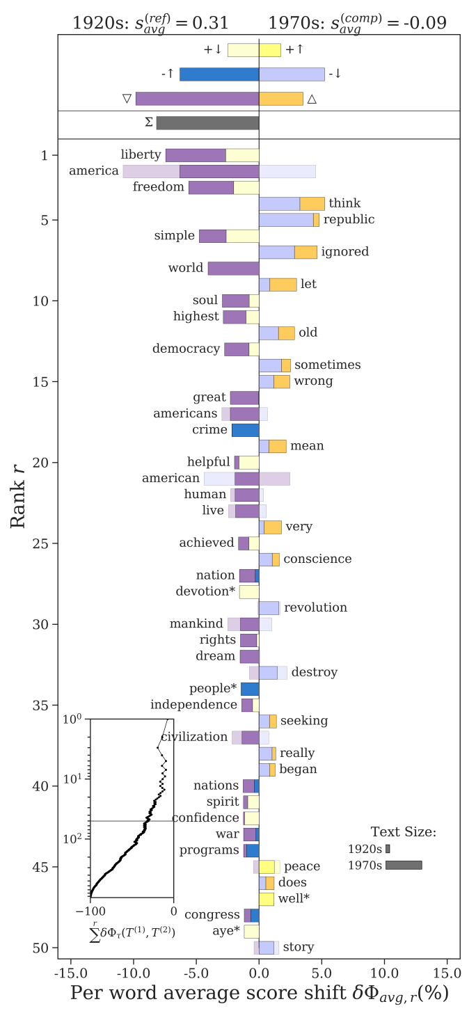
Visualizing words: Word Shift Graphs
Visualizing networks: spring layout

Visualizing networks: known underlying structure

Random things I thought might be helpful
Colors
Image filetypes
							plt.savefig("my_figure.png", dpi=300)

							# great to import in Inkscape or Adobe Illustrator
							plt.savefig("my_figure.svg")

							plt.savefig("my_figure.pdf")

							# this does not work :(
							plt.savefig("my_figure.eps")
Plot coding style: use functions
							def PlotSomethingNice(ax, data, param="xy"):
								...
								...

							def PlotAnotherNiceThing(ax, data, param="xy"):
								...
								...

							fig, axes = plt.subplots(2, 2)

							PlotSomethingNice(axes[0][0], subset1, param="first part")
							PlotSomethingNice(axes[0][1], subset2, param="second part")
							PlotAnotherNiceThing(axes[1][0], df, param="do this")
							PlotAnotherNiceThing(axes[1][1], df, param="do something else")
Large data
Problem 1: since every data point is an object, Matplotlib gets VERY slow for large amounts of data.
Problem 2: figure files also get VERY large because of this.
Solution 1: subsample your data.
less_data = lots_of_data.sample(frac=0.05, random_state=42)
Solution 2: rasterize your figures and save as .png.
Summary
Matplotlib + Seaborn offers both high abstraction and excessive detail.
Use known visual metaphors and de-clutter your plots for maximum clarity.
Whenever you do something unexpected in your visuals (resampling or excluding data, truncating axes), DESCRIBE IT in the text.